Route Cost Follows Density, Not Scale

Introduction

A multi-branch operator adds a customer across town and books the revenue. The revenue is real, but so is a cost that never shows up on the invoice: the time a technician now spends driving to reach it. In field service, the price of a stop is not just what happens at the stop. It is set by where the stop sits relative to every other stop on the route. That is why two operators of the same size can run very different unit costs, and why growth that scatters accounts across a map can quietly raise the cost of serving all of them. Route cost follows density, not scale.

• Drive time per stop falls with the square root of density. Under the standard routing approximation, the local driving distance per stop is proportional to 1 over the square root of density, so to halve it you need roughly four times the density in the same area. It is a scaling shape, not an exact law.
• Cost is time and labor, not the mile.The expensive input on a route is the technician’s hour, not the gallon of fuel. A service technician’s wage runs the meter every minute of windshield time, which is why cutting drive time per stop is the lever.
• Density is not the same as scale. Adding scattered accounts adds scale without density and can raise unit cost; adding accounts that cluster raises density and lowers it. More customers only help if they make the map denser.
• Software exploits density; it does not create it. A good solver moves a route closer to the theoretical floor, but the floor itself is fixed by the book and the territory. Density is built in sales geography and territory design, and only then optimized.

Why the cost of a stop depends on your other stops

Split the cost of a service visit into two parts. There is the service time, the fixed minutes a technician spends actually doing the work at the address, and there is the drive time, the windshield time between the previous stop and this one. Service time is roughly constant per visit. Drive time is not: it depends entirely on how close the next stop is, which depends on how many other customers you have nearby. A dense book means the next job is minutes away. A sparse book means it is across town. The same technician, doing the same work, produces very different economics depending on the geography of the route around each stop.

This is why a single average cost per stop can mislead as badly as a single average anything. Two branches with identical service work can post different unit costs purely because one serves a dense metro and the other a scattered rural territory. Before you conclude that one branch is run better, you have to separate the part of the cost that is geography from the part that is execution. The geography, it turns out, obeys a rule precise enough to put a number on.

The square root of density: what the routing math says

The rule comes from a result proved in 1959. Beardwood, Halton and Hammersley showed that the length of the shortest round trip through N stops scattered across a territory of area A grows in proportion to the square root of N times A. Divide that tour length by the number of stops and you get the practical form: the driving distance per stop is proportional to the square root of area over stops, which is one over the square root of density. Daganzo (1984) extended this into a working fleet model, splitting a route into a line-haul term that carries a truck from the depot out to its territory and a local term that carries this same square-root-of-density shape. It is now a mature method, used across the continuous-approximation literature as a check on full-blown route solvers.

The consequence is concrete and a little counterintuitive. Because the relationship runs through a square root, the returns to density diminish: each doubling of density cuts drive distance per stop by only about 30 percent, and to cut it in half you need roughly four times the density. The scope has to travel with the rule, because it is an approximation, not a law of nature. It is asymptotic, meaning it describes large routes better than tiny ones; it assumes customers are spread evenly and distances are straight-line, so real, clustered books beat it and real roads (which add perhaps 20 to 40 percent of circuity) inflate it; and it describes driving only. It is best read as the shape of the curve, not an exact multiplier, and the right unit is local density in each service zone, never one global average for the whole company.

Where route cost actually goes: time and labor, not the mile

The square-root rule matters because of where route cost actually sits. The expensive input is time, and time is labor. A pest-control technician earns a median of about $21.75 an hour, and a grounds and landscaping worker about $19.27 an hour, before the benefits and overhead that push the fully loaded figure materially higher. Every minute of windshield time is billed against that rate whether or not the truck is doing anything productive. Set that against the vehicle: the IRS standard mileage rate, about 70 cents a mile, bundles fuel, maintenance and depreciation into a single number and still excludes the driver entirely. The mile is cheap; the hour is not.

The heavy-truck world makes the same point at a larger scale, and it has to be borrowed carefully. The American Transportation Research Institute puts the marginal cost of operating a truck at about $2.34 a mile in 2025, with driver wages and benefits among the largest and fastest-growing line items. That dollar figure is a Class-8 long-haul number and does not transfer to a light service van: it is cited only as evidence of the mechanism, that route cost is dominated by time-linked and labor-linked items, not by the marginal mile. The lesson for a field-service operator is the same one the arithmetic keeps returning: the thing worth cutting is the drive time per stop, because that is the thing consuming the expensive hour.

Density versus scale: why scattered growth raises unit cost

This is where the strategy diverges from intuition. It is natural to assume a bigger operator is a cheaper one, that scale lowers unit cost. In routing, that is only true if scale arrives as density. The distinction is the one Caves, Christensen and Tretheway drew between economies of density and economies of scale: density is more output in the same territory, scale is more territory. Adding a thousand customers clustered inside your existing service areas raises density and lowers cost per stop. Adding the same thousand scattered across new, thinly served geographies raises scale without density, and can raise cost per stop, because each of those accounts sits far from the next.

For an acquisitive, multi-branch operator this is the whole game. A roll-up that buys books which overlap and infill its existing territories is buying density, and the combined route economics improve. A roll-up that buys books in scattered new markets is buying scale, and unless it reaches serviceable density in each one, the unit economics do not follow the revenue. The same acquisition can be accretive or dilutive to route cost depending entirely on where the customers are. Growth is not automatically leverage; clustered growth is.

We ran the numbers: a reproducible density simulation

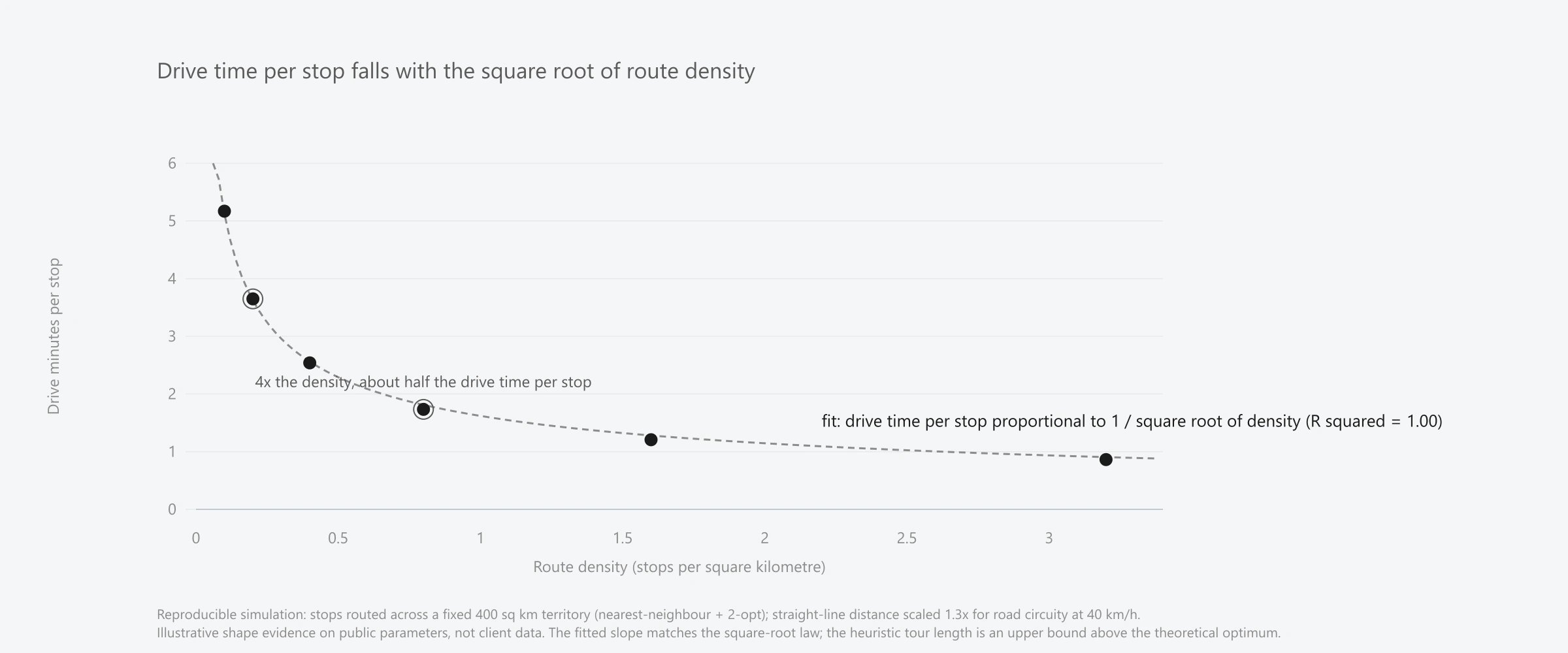
To see the shape on something more tangible than a formula, we ran a reproducible simulation, and it is the chart at the top of this page. Stops are placed across a fixed 400 square-kilometre territory at rising density, routed with a near-optimal solver (a nearest-neighbour construction improved by 2-opt), and straight-line distances are scaled by a 1.3 times road-circuity factorat a 40 kilometre-per-hour service speed. Everything is seeded, so the figure is reproducible to the digit, and every parameter is public. It is illustrative shape evidence, not any operator’s real minutes, and it uses no client data.

The result tracks the theory closely. Across the swept range the drive time per stop falls from about five minutes at low density to under a minute at high density. A fit to a one-over-the-square-root-of-density law tracks the simulated points with an R-squared of 0.999, and on logarithmic axes the relationship is a straight line with a slope of about negative 0.52, against the theoretical negative 0.5. In plain terms, quadrupling the density roughly halves the drive time per stop, exactly as the square-root rule predicts. One honesty note travels with it: the solver is a heuristic, so its tour lengths are an upper bound that sits a little above the theoretical optimum (its constant runs near 0.79 against the ideal 0.71 and trends toward it as density rises), which is why the validation rests on the slope of the curve, not its exact height. A separate run makes the density-versus-scale point physical: a book whose stops are clustered rather than spread uniformly is about 25 percent cheaper in drive distance per stop at the same overall density, because what the truck actually experiences is the local density, not the company-wide average.

Where the density benefit stops: the service-time floor

Density is powerful, but it is not unbounded, and the honest version of the thesis says where it stops. The drive time per stop falls toward zero as density rises, but the total time per stop cannot, because the fixed service time at each address is a floor the routing never touches. In the same simulation, if a visit takes fifteen minutes of on-site work, rising density lifts a technician from roughly twenty-four to about thirty stops in an eight-hour day. If the visit takes thirty-five minutes, the same density gain moves the needle only from about twelve to thirteen. The on-site time is a disclosed, swept assumption here, not a claim about any real operator, but the structural point is exact: the denser your book, the more the day is governed by the work itself and the less by the driving, which is the goal.

Other constraints bend the curve the same way. Tight appointment windows, vehicle or route capacity, and skill-based routing (the right technician for the job) all limit how fully a solver can convert density into saved drive time. Figliozzi and others have modeled how these constraints raise the achievable route length above the idealized minimum. None of this overturns the rule; it scopes it. Density remains the dominant lever on the drive component of per-stop cost, with a floor set by the work and a ceiling set by the constraints.

What software can and cannot do, and what density means for value

This is the boundary a vendor has to state plainly. Route optimization software is real leverage: a better solver moves a live route closer to the theoretical lower bound, and standard benchmark librariesexist precisely to measure how close a solver gets. But the lower bound itself is fixed by the configuration, by N, the area, and the geometry of the book, which are properties of the customers and the territory, not of the software. A solver can only approach the shortest tour the book’s own geometry allows; it cannot manufacture density that is not there, and the square-root rule is the shape of the idealized uniform case, not an exact floor. So the honest claim is narrow: software exploits the density you already have. It does not create density. Density is built earlier, in sales geography, in territory design, and in the discipline to set minimum-density thresholds before serving a new area. Ardenus sits on top of the systems an operator already runs and helps measure and act on exactly those inputs, but no routing tool, ours included, has been shown here to deliver a specific saving; the link from density to cost is the routing mathematics, not a claim about any product.

The reason this reaches the boardroom is that route density is where operations become margin. Lower drive time per stop is lower cost per stop, which is higher gross margin on the same revenue, and margin is one of the levers that a rigorous buyer prices. The connection has to be drawn carefully: density moves the margin and therefore the value level, not the valuation multiple directly, a distinction we develop in the companion essay on why valuation follows revenue quality, not revenue. It also compounds with the rest of the book. A denser route is cheaper to serve and, because the technician is nearby, easier to serve well, which feeds the retention economics we cover in why churn is a distribution, not a number. The through-line is the one this essay began with: build density in the book and the territory, measure it honestly, and let the routing follow. You can read more of our research on the Ardenus articles hub, or see the platform itself on the technology page.