Timing Lawn-Care Capacity with Growing Degree Days

Introduction

Every spring a lawn-care operator makes the same bet: it decides when the season starts. Crews are hired, materials are pre-bought, and the first round of visits is scheduled, usually against a date on the calendar that worked last year. But the lawn does not read the calendar. Grass greens up, weeds germinate, and insects emerge when the ground has accumulated enough warmth, and that happens on a different date every year and weeks apart from one market to the next. The operator that staffs to a fixed date is early in a cold spring and late in a warm one, and wrong in opposite directions across a multi-branch footprint on the very same week. The season follows growing degree days, not the calendar.

• The season starts on a temperature, not a date. Below a base temperature, plant and insect development effectively stalls, so the accumulated heat above that base, the growing degree days, tracks progress toward the events an operator has to serve better than the day of the year does.
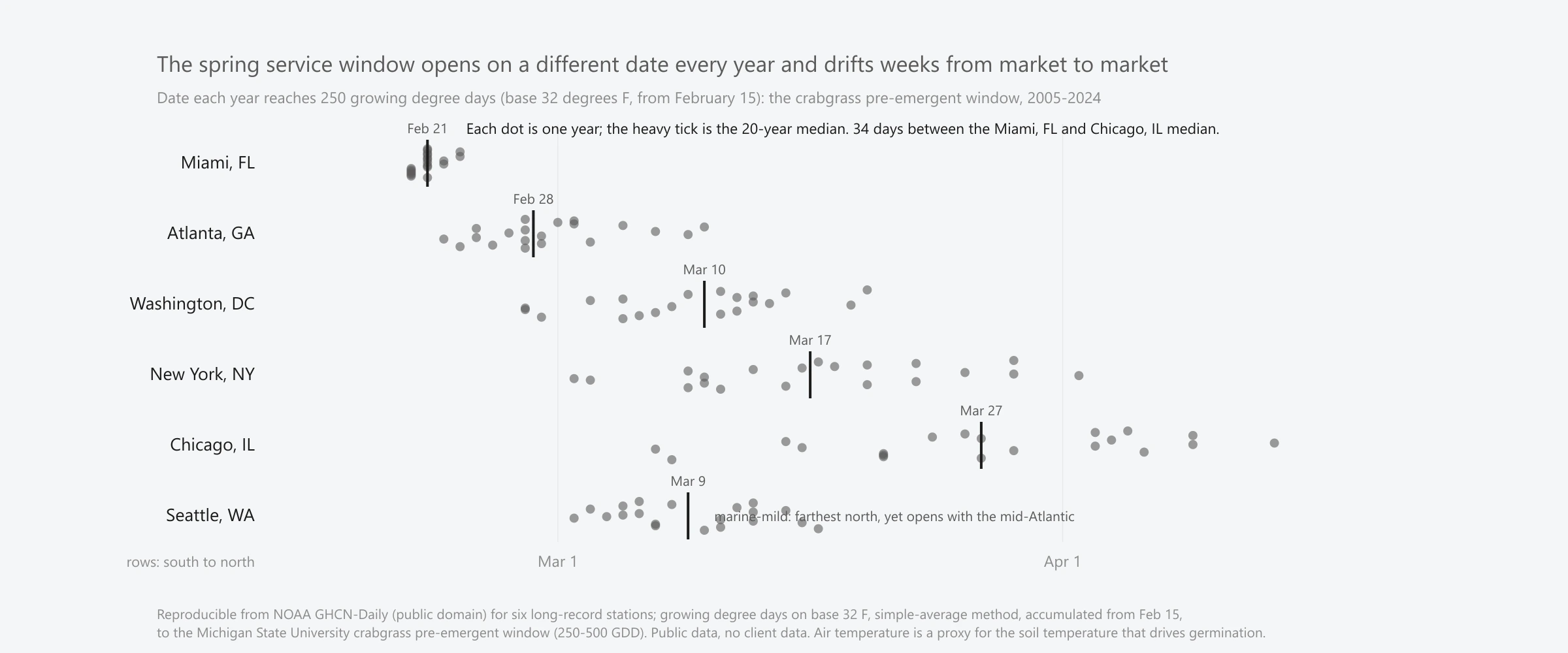
• The opening date moves by weeks. In our computation on public weather data, the spring pre-emergent window at one city swings across a 31-day range from year to year, and its median opening date drifts 34 days across a south-to-north footprint. Same service, very different weeks.
• It is heat, not latitude. A latitude rule fails too: marine-mild Seattle, the farthest north of the markets we tested, opens its window with the mid-Atlantic. Only accumulated temperature captures that, which is why a regional calendar is not enough.
• Reconcile the plan against a live reading. The fix is not a better fixed date; it is comparing a seasonal plan against a live accumulated-degree-day reading each spring and moving crews and materials to the market where the window is actually opening.

When does the lawn-care season actually start?

The honest answer is that it does not start on a date at all; it starts on a threshold. What a customer sees as green-up, and what an agronomist tracks as the moment to act, is the result of heat accumulating day after day until the biology crosses a line. A run of warm days in February pulls the season forward; a cold, late spring pushes it back. Two neighboring years in the same town can differ by weeks, and two towns a few hundred miles apart can differ by more than a month in the same year. A calendar is a guess at the average of that variation, and the average is exactly the thing an operator planning fixed, short-term capacity cannot afford to be wrong about.

The stakes are set by how seasonal the work is. Landscaping-services employment in the United States swings from roughly 748,000 jobs in January to about 1,014,000 by the middle of 2024, a swing of some 266,000 jobs, about 36 percent of the workforce, added and shed inside a single year (Bureau of Labor Statistics series CEU6056173001, not seasonally adjusted). Capacity like that is built and released on a schedule, and the schedule is only as good as its guess about when demand actually arrives. That recurring swing is calendar-predictable in the gross, but the money is made or lost in the marginal weeks at the front of the season, where the timing is not a calendar fact.

What growing degree days are, and why they beat the calendar

A growing degree day is a simple accountant of heat. Take the day’s high and low temperature, average them, subtract a base temperature below which development effectively stops, and, if the result is positive, that is the day’s contribution. Add those contributions up from a start date and you have accumulated growing degree days, a running total that stands in for biological progress far better than the number of days elapsed. It is a deliberately coarse model, and its power is that it is coarse: one number, computed from thermometers everyone already has.

The scope has to travel with the method, because it is an approximation, not a biological law. The same idea is, as one classic treatment put it, one equation with two interpretations: the base temperature, the averaging method, and whether an upper cap is applied all change the total, so a growing-degree-day figure is meaningless without its recipe attached. Different organisms use different bases. And the air temperature a weather station records is only a proxy for the soil temperature and moisture that actually trigger germination, so a dry or false spring can break the relationship. Growing degree days are necessary for good timing, not sufficient for it; they narrow the window from a month to a matter of days, and the agronomy fills in the rest.

Timing the pre-emergent window by accumulated temperature

The clearest lever is the pre-emergent crabgrass application, because it has to land in a window that opens and closes on heat. A pre-emergent forms a barrier before the weed germinates; apply it too late and the crabgrass is already up and the product cannot control it, apply it too early and the barrier can break down before the threat arrives. University turf programs express that window in growing degree days rather than dates for exactly this reason. The Michigan State University GDD Tracker, calibrated by Calhoun, places the optimal window at 250 to 500 growing degree days on a base of 32 degrees Fahrenheit, using the simple-average method and accumulating from February 15. The peer-reviewed literature ties the same event to accumulated heat: Fidanza, Dernoeden and Zhang showed smooth crabgrass emergence is keyed to degree-day accumulation rather than to a fixed calendar date.

The old forsythia-in-bloom folklore is really this same signal read off a different instrument: the shrub responds to the same accumulated heat, so its bloom coincides with the window. The growing-degree-day model just formalizes the coincidence and puts a number on it. Precisely because the number carries a specific base, method, and start date, it is portable across markets in a way a date is not, and it is auditable: given the same weather record, two people compute the same window.

How much the window moves, by year and across a footprint

To put real numbers on the movement, we computed it, and the result is the chart at the top of this page. Using the public NOAA GHCN-Daily record, we pulled daily high and low temperatures for six long-record stations on a south-to-north gradient, from Miami to Seattle, over the twenty years from 2005 to 2024, required each spring to be at least 98 percent complete, and computed the date each year first reached 250 growing degree days on base 32 from February 15: the moment the pre-emergent window opens. Everything runs from a committed public-domain data subset, so the figure is reproducible to the day, and it uses no client data.

The variation is large in both directions. At a single station, New York, the window opens as early as March 2 and as late as April 2, a 31-day range from year to year around a median of March 17. Across the footprint the median opening date spans 34 days, from February 21 in Miami to March 27 in Chicago. The same calendar date is a completely different biological moment from one market to the next: by April 1 the accumulated total is 1,937 growing degree days in Miami, whose window closed weeks earlier, but only 324 in Chicago, which is just crossing into its window. And latitude alone does not save you, because it is heat that is accumulating, not degrees of latitude: Seattle, farthest north of the six, opens around March 9, right alongside the mid-Atlantic, because its mild marine winter banks heat that a continental winter at the same latitude does not. An 86 degree Fahrenheit upper cap, a common refinement to the method, barely moves any of this, shifting the median opening by a day or less, so the pattern is not an artifact of one modeling choice.

Growing degree days on the pest side: insect emergence

The same clock runs on the pest-control side of a field-service book, which is why this is not only a lawn story. Insect development is temperature-driven in the same way, and integrated pest management has used degree-day models for decades to time treatments to a target life stage rather than to the calendar. The distinction to keep straight is the base temperature: many insect models accumulate on a base of about 50 degrees Fahrenheit, not the 32 the crabgrass turf model uses, and each pest carries its own developmental thresholds and calculation method. The two conventions are genuinely different quantities and must never be interchanged, but the principle is identical: heat accumulates toward a threshold, and the threshold, not the date, is what you schedule against.

This is now operational, not theoretical. The USA National Phenology Network publishes short-term phenology forecasts that apply accumulated degree days to time the emergence of specific insect pests, the same machinery pointed at a different organism. For a multi-branch operator running both trades, the lesson generalizes: the demand for a timed treatment, lawn or pest, opens on a temperature threshold that moves, and the branch that watches the accumulation is ready when it opens.

Reconciling a seasonal plan against a live degree-day nowcast

Knowing the window moves is only useful if it changes what you do. The move is to treat the seasonal plan as a baseline, not a schedule, and reconcile it each spring against a live reading of accumulated heat, the kind the USA-NPN publishes as public accumulated-degree-day maps updated daily. When the accumulation is running ahead in the south and behind in the north, the plan bends: crews and materials sequence to the markets whose windows are opening first, pre-emergent is pre-bought against the nowcast rather than the calendar, and the front of the season is worked in the right order instead of all at once.

The reason a fixed date cannot substitute for this is that the residual error of any fixed date is irreducible, not a matter of learning your market. In the same computation, we gave every branch the best fixed date it could possibly have, its own twenty-year median opening date, and then asked how often that date still missed the live 250-to-500 window. It missed in 43 percent of branch-years, and in a year it missed, the fixed date fell a mean of 5.6 days outside the window, almost always by being too early in a year that opened late. Even perfect knowledge of your average leaves you outside the window nearly half the time, because the variation is in the weather, and only a live reading of the weather catches it.

What the public data proves, and what it does not

It is worth being exact about what this evidence supports. It shows, on public data anyone can re-run, that the timing of a spring service window is governed by accumulated temperature and moves by weeks year to year and market to market, and that a calendar or a latitude rule cannot track it. It does not show, and this essay does not claim, a dollar figure for the cost of getting the timing wrong, or a demand curve. Growing degree days gate the timing of the window, not the size of demand, which also turns on contracts, price, marketing, and workable-weather days. Air temperature is a proxy for the soil that actually drives germination, and the stations are first-order airport records that can run warmer than a shaded turf canopy. Those are real limits, and the honest thesis lives inside them: the signal is the timing, and the timing is real.

That is also the boundary a vendor has to state plainly. Software does not create demand or capacity, and it does not move a threshold; what it can do is measure the accumulation against each branch and each service, and make the reconciliation routine instead of heroic. Ardenus sits on top of the systems an operator already runs and helps turn the public degree-day signal into a staffed plan, but no result, saving, or forecast accuracy is attributed to Ardenus here; the link from temperature to timing is agronomy and the public record, not a claim about any product, and no client or first-party data appears anywhere in this essay.

The reason this reaches the boardroom is that timing capacity to the season is where a lawn book’s revenue becomes durable. A season that is staffed to the real window is served on time and served well, which shows up as more predictable seasonal revenue, the kind of revenue quality a buyer prizes, a connection we develop in the companion essay on why valuation follows revenue quality, not revenue. It compounds with the rest of the book, too. A service delivered in its window is one that does not become an early cancellation, which feeds the retention economics in why churn is a distribution, not a number; once the season opens, serving the surge efficiently is the subject of our essay on why route cost follows density, not scale; and reconciling a plan against weather depends on clean, well-joined service history, the theme of the negative effects of dirty data. The through-line is the one this essay began with: read the season off the temperature, not the calendar. You can read more of our research on the Ardenus articles hub, or see the platform itself on the technology page.