What It Costs to Serve a Customer

Introduction

Most multi-branch pest-control and lawn-care operators price with one hand while spending with the other. The price on a recurring contract is set as a flat annual or quarterly rate, a per-visit charge, or a rate per square foot, and it barely varies from one customer to the next. What it costs to serve those customers is not flat at all: a compact property on a dense route a few minutes from the last stop and a sprawling one at the end of a long drive can carry the same price and consume wildly different amounts of a crew’s day. When price is uniform and cost to serve is not, the flat rate quietly over-charges the cheap-to-serve customer and under-charges the expensive one, and the margin the business thinks it is earning is an average that is true of almost no one. The fix is not a gut feel about which accounts are heavy; it is to compute what each job actually costs to serve and to set price as a function of that cost.

• A single flat rate is a pooling price. Set one price across customers whose cost to serve spans a wide band and it sits above what the cheap-to-serve customer should pay and below what the expensive one should, so contribution margin leaks in both directions at once.
• Cost to serve is computable, not a guess.Time-driven activity-based costing turns a resource’s cost and a job’s minutes into a defensible unit cost: a capacity cost rate times the time each task consumes. It is a model with disclosed assumptions, not a measurement, but it is auditable and reproducible.
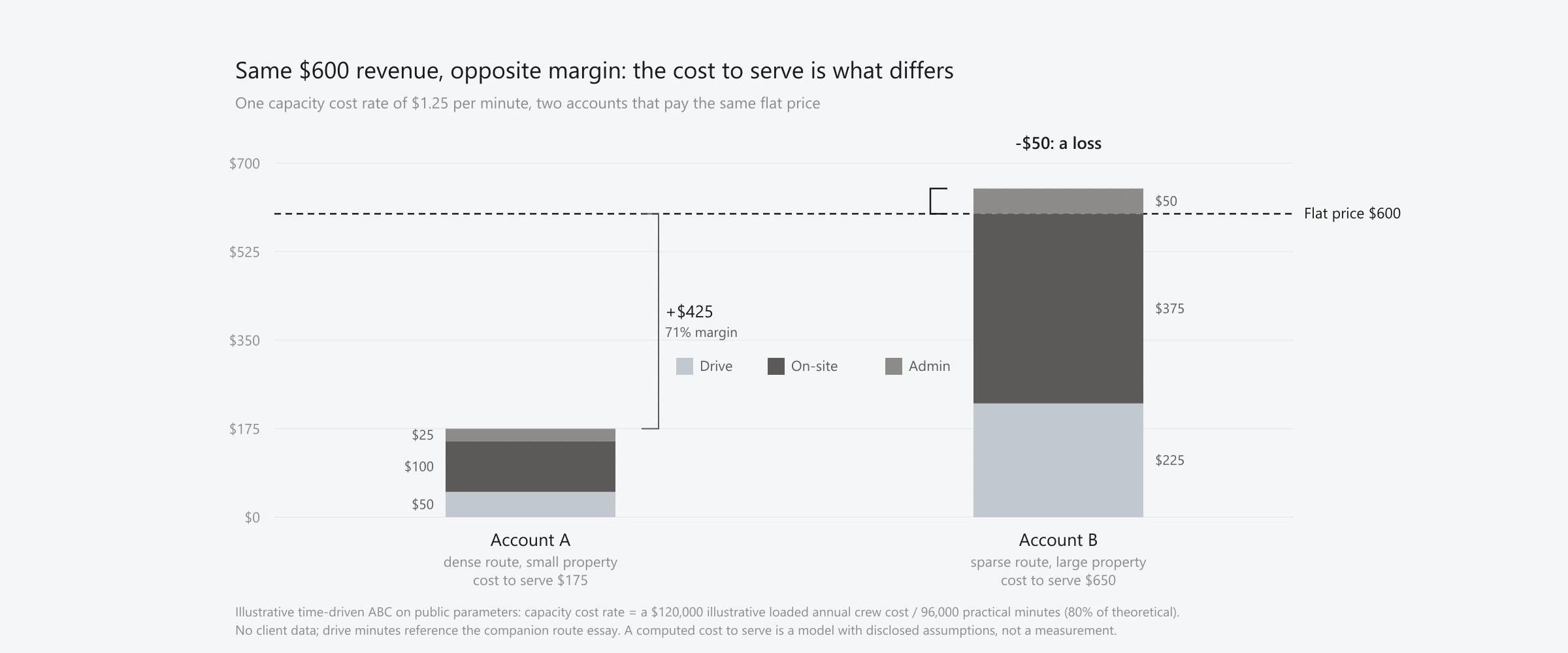
• Two customers, same price, opposite margin. In the reproducible example on this page, two accounts pay the same $600 and one shows a margin of about 71 percent while the other posts a loss, purely because their cost to serve differs. Same revenue is not same profit.
• Then price to the cost you computed. Once cost to serve is on the table, the pricing moves are ordinary and well-documented: a value-based floor, segmented plans and good-better-best, minimums and surcharges for the expensive tail, or re-engineering the relationship so the cost itself comes down.

Why a flat rate is a pooling price

The instinct to price on cost is right; the usual execution is not. Cost-plus pricing takes a unit cost and adds a markup, but the unit cost of a service depends on volume and mix, and volume depends on the price being set, so the method is circular: you need the price to know the cost you are marking up. Worse, in field service the “unit cost” that gets marked up is almost always an average across the whole book, and an average cost applied to a heterogeneous book is a pooling price. Charge every customer the mean cost to serve plus a margin and the rate lands above what a cheap-to-serve customer costs and below what an expensive one costs. The cheap account is over-charged and becomes a target for a competitor who has done the arithmetic; the expensive account is under-charged and is subsidized by the rest of the book.

That is not a stable place to sit. A uniform price over a spread of costs is, in the language of insurance and market design, a pooling equilibrium, and pooling prices tend to unravel toward their high-cost tail: the customers who are cheapest to serve have the most incentive to leave for a keener rate, which raises the average cost of the customers who remain, which raises the price the book needs to break even, which pushes the next-cheapest cohort to the exit. This equilibrium logic is what justifies pricing to cost to serve, and it is stated as theory, not a measured claim about any operator; it is deliberately a statement about the pressure on a single price, not about the shape of profit across a whole book, which is a separate question with its own essay. The point that carries is narrower and firmer: when cost to serve varies and price does not, a flat rate is leaving margin on the table in both directions, and the only way to know how much is to compute the cost.

How to cost one unit of service

The tool for computing it is time-driven activity-based costing, introduced by Kaplan and Anderson as a simpler successor to traditional activity-based costing. It rests on a two-step formula that is easy to audit. First, compute a capacity cost rate: the cost of the resources supplied to do the work divided by the practical capacity of those resources, which yields a cost per minute of productive time. Second, cost any job as that capacity cost rate multiplied by the number of minutes the job actually consumes. A field visit is not one number but a sum of tasks, so the minutes are expressed as a time equation, a base time plus increments for the things that make a job longer: a larger property, a harder access, an added service, a mixed application. The strength of the method is that it absorbs that heterogeneity without re-surveying staff for every account, and the same machinery has been shown to work on real books in adjacent industries, for instance a wholesale distributor whose order-handling cost was modeled with multi-term time equations rather than a single average.

One number in that formula does most of the work and has to be disclosed: the practical capacity in the denominator. It is not the theoretical maximum of minutes in the year; Kaplan and Anderson recommend using roughly 80 to 85 percent of theoretical capacity, reserving the rest for breaks, travel between the productive tasks, training, and the ordinary friction of a working day. That convention is an assumption, and it scales every unit cost directly: a lower practical-capacity figure raises the cost per minute and therefore the computed cost of every job, and a higher one lowers it. A cost to serve is only as honest as the capacity assumption behind it, which is why a computed cost to serve is a model with disclosed assumptions, not a measurement. What the method buys, in exchange for stating those assumptions out loud, is a cost that attaches to the real drivers of a job instead of a companywide average, and a cost-to-serve view in which the cost of serving a customer is traced to that customer rather than smeared across all of them.

Two accounts, same price, opposite margin

The chart at the top of this page makes the mechanism concrete with a fully reproducible computation on public, illustrative parameters, and no client data anywhere. Start with one capacity cost rate. Take an illustrative fully-loaded cost of a single crew of $120,000 a year, and a practical capacity of 96,000 minutes, which is 80 percent of a theoretical 120,000 minutes; the capacity cost rate is $120,000 divided by 96,000, or $1.25 a minute. Now take two recurring accounts that pay exactly the same flat price of $600 a year, served quarterly. Account A sits on a dense route with a small property: about 35 minutes a visit, which at four visits and $1.25 a minute is a cost to serve of $175, for a margin of $425, or 71 percent. Account B sits on a sparse route with a large, complex property: about 130 minutes a visit, which is a cost to serve of $650, more than the price, so the account loses $50 a year. The drive portion of those minutes is the province of the companion essay on why route cost follows density, not scale, and it is referenced here rather than re-derived; what this essay adds is the rest of the job, the on-site and administrative minutes, and the pricing that should follow.

The lesson is in the identical prices and the opposite outcomes. Same revenue is not the same profit; one account is a 71 percent margin and the other is a loss, and the flat $600 hid the difference completely. It is worth stating exactly what this example is and is not. It is a mechanism demonstration with two accounts, built to show that a flat price straddling different cost-to-serve profiles produces different margins; the specific figures are illustrative public parameters, not a measurement of any operator’s book. It is not a claim about how many customers in a real book are unprofitable or how profit is distributed across the whole book, which is a genuinely different question, the shape of profit across all accounts, and the subject of a separate companion essay. Here the unit is one customer, used forward: given the job, compute the cost, then set the price.

How to price to cost to serve

A computed cost to serve is an input to a pricing decision, not the decision itself, because cost sets a floor and value sets the ceiling. The other side of the same discipline is to understand what a customer actually values, so that price tracks the value delivered rather than only the cost incurred; a job that is expensive to serve but highly valued can carry its price, while a cheap-to-serve commodity visit cannot be marked up just because a competitor is absent. Between the cost floor and the value ceiling, the moves are ordinary and well-documented. A useful way to sort a book is the classic net-price-versus-cost-to-serve grid: accounts that realize a high net price at a low cost to serve are kept as they are; low net-price, low-cost accounts can often be repriced; high-cost accounts that still clear a fair price are fine; and high-cost accounts at a low realized price are the ones to reprice, re-engineer, or, as a last resort, let go.

The instruments for doing that without renegotiating every contract are familiar: segmented plans and good-better-best tiers, minimums that floor the small, expensive-to-reach job, and surcharges for the drivers that actually add cost, a distant property, an oversized lot, an extra service. It helps to remember that the price a business realizes is not the price on its rate card: once discounts, concessions, and the cost of serving each account are netted out, the realized pocket price varies account to account far more than the list price suggests, and two customers on the same published rate can net very different margins. Often the best move is not to reprice at all but to re-engineer the relationship so the cost to serve comes down, by consolidating visits, adjusting frequency to what the property needs, or sequencing the account into a denser part of the route. Pricing to cost to serve is not a single lever; it is the discipline of letting a computed cost, rather than an average, decide which of these moves each account needs.

Assumptions and limits

The honesty of this method is in its disclosures, so they belong in the open. A computed cost to serve is a model output, contingent on choices, not an observed fact: the practical-capacity percentage, which costs are counted as the cost of resources supplied, and the form of the time equation all move the answer, and a different analyst with different conventions will get a different cost. The time equations are estimates, built from observation and judgment and assumed to be linear in their drivers, when real jobs have thresholds, learning effects, and interactions a straight line does not capture; the method is built to be approximately right rather than precisely wrong, and that tolerance has to travel with the number. A TDABC cost to serve is also a fully-loaded allocation, not an incremental or avoidable cost: the fixed cost of capacity that is already paid for does not disappear when a single account leaves, so pricing or dropping a customer as though the allocated cost were avoidable can mislead. Idle, unused capacity should be surfaced as its own line and not loaded onto customers, or every cost to serve is inflated.

Two limits are specific to this trade. Capacity and cost are assumed stable over the costing period, and pest-control and lawn-care demand is strongly seasonal, so the rate computed against a full-year capacity differs from one computed against a compressed peak, and the period has to be stated. And the evidence for the method comes from services, logistics, and wholesale settings, not from pest control or lawn care; the mechanism transfers, but no one should read the canonical examples as field-service data. The claim this essay defends lives inside those limits: that cost to serve varies, that it can be computed with a disclosed model, and that a flat price over a spread of costs leaves margin unclaimed. That a repricing will capture the margin is not guaranteed, because customers can leave and competitors can undercut; the market response is an assumption, not a mechanical certainty, and every margin figure here is an analytical implication under stated assumptions, not a measured result.

What this means for the operator

For a multi-branch operator, the practical program is small and concrete: build a capacity cost rate for a crew, write a time equation for a visit that includes the drivers that actually move cost, and let the computed cost to serve, rather than a companywide average, inform the price on each account and each plan. Doing that turns pricing from a single posted rate into a deliberate match between what a job costs and what it is worth. It also draws a clean line to the neighboring questions: the drive component of that cost is the subject of the essay on route cost and density; the shape of profit once every account’s cost to serve is summed across the whole book is a separate question for a separate essay; and the reason margin discipline reaches the boardroom at all is that steadier, higher-quality margin is what a buyer pays a premium for, the argument of why valuation follows revenue quality, not revenue. Pricing to cost to serve also protects the book from the wrong kind of loss: an account priced below its true cost is a slow cancellation waiting to be rationalized, which connects to why churn is a distribution, not a number, and the whole exercise depends on clean, well-joined service records, the theme of the negative effects of dirty data.

The boundary a vendor has to state is plain. Software does not set the price, and it does not decide which accounts to reprice, re-engineer, or keep; those are the operator’s calls, and the value of a computed cost to serve is only as good as the assumptions disclosed with it. What a data and intelligence layer can support is that computation: assembling the capacity cost rate, keeping the time equations current, and attaching a cost to serve to every account so the pricing conversation starts from a number instead of a hunch. Ardenus is built for that measurement layer and sits on top of the systems an operator already runs, but no result, saving, or forecast is attributed to Ardenus here; the method is the public record of cost accounting and pricing, and no client or first-party data appears anywhere in this essay. You can read more of our research on the Ardenus articles hub, or see the platform itself on the technology page.